
Quantum optics
The TDC-A covers the standard measurements around single-photon detectors, such as coincidence counting, g²(τ) antibunching measurements, and the characterization of photon-pair sources.
Exvi Technologies builds user-friendly, plug-and-play scientific instruments for precision timing. Our first product, the TDC-A, is a compact USB time tagger for photon counting and event-timing applications. All Exvi products come with easy-to-use software and a programming interface for automated measurements.
The TDC-A is Exvi's low-cost, picosecond-resolution USB time tagger. View TDC-A →
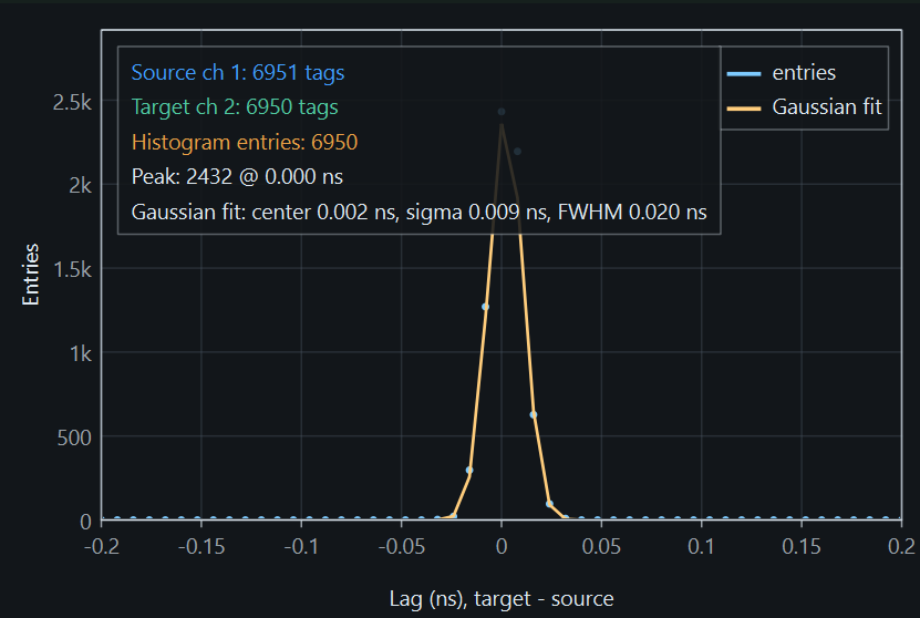
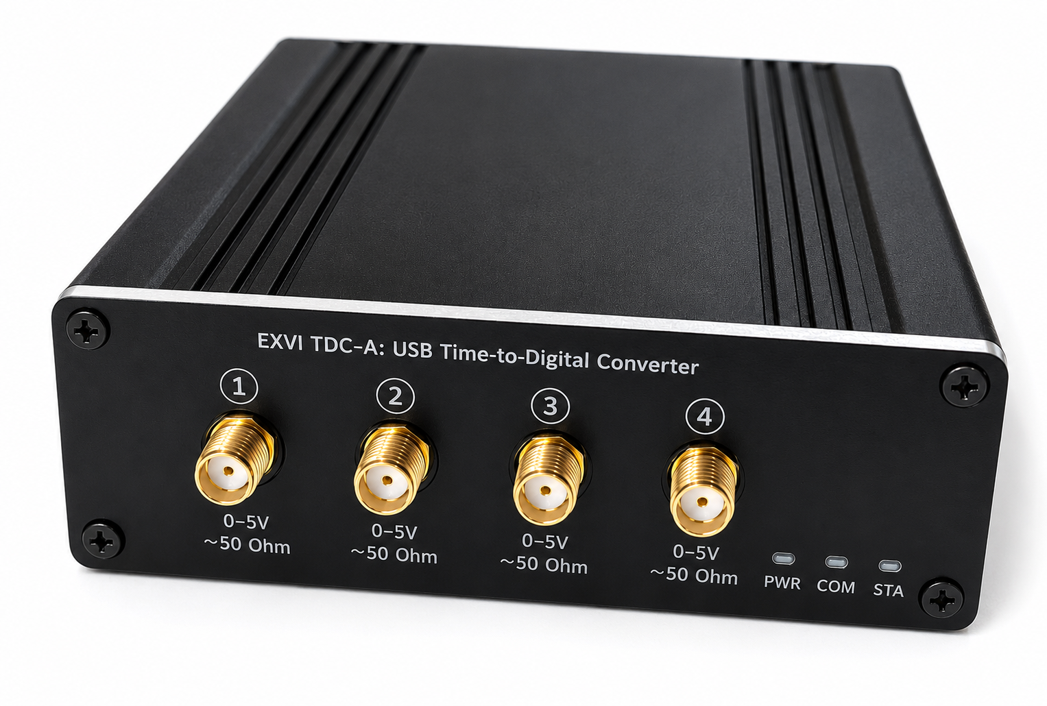
The TDC-A covers the standard measurements around single-photon detectors, such as coincidence counting, g²(τ) antibunching measurements, and the characterization of photon-pair sources.
Lidar and fluorescence-lifetime measurements (TCSPC / FLIM) both record the delay between a reference pulse and a detector event. A time tagger measures this delay directly, at picosecond resolution.
A time tagger is also a general-purpose tool for electronic timing. It can measure the period, jitter, and drift of a clock signal, or record asynchronous pulses from a device under test for later analysis.
Compact USB time tagger for counts, streaming, correlation, and other timing-heavy measurement workflows.
The TDC-A is a four-channel USB time tagger: 22 ps typ. (40 ps max) RMS jitter, 4 ps bin width, up to 100 MCPS per channel. It streams raw timestamps to the host, where the GUI or the Python & C++ API handles counting, correlation, and analysis.
$2,370
Indicative price only, not an offer for sale — the TDC-A is not yet certified and is not currently offered for general sale.
Price per device, excluding shipping and sales tax. Quantity and academic discounts available. See pricing policy.
Coming soon →Schematic overview — not to scale. The clock port can carry a 10 MHz reference or a dedicated synchronization signal for multi-unit setups.
Preliminary — typical values from pre-production units, subject to change pending final characterization.
*Jitter may be added for pulse spacing of less than 20 ns.
**Bin width is set in software, down to a minimum of 4 ps.
The TDC-A is the first product. If your application needs more channels, a different form factor, or a specific feature, tell us — it shapes what we build next.
TDC-A is controlled through exvi.timing — Exvi's timing software, with a desktop GUI plus a Python & C++ API and drivers, on Windows and Linux. Go to software →
Every Exvi instrument ships with the software to run it: drivers, a desktop GUI, and a Python & C++ API. exvi.timing is the package for the TDC-A time tagger.
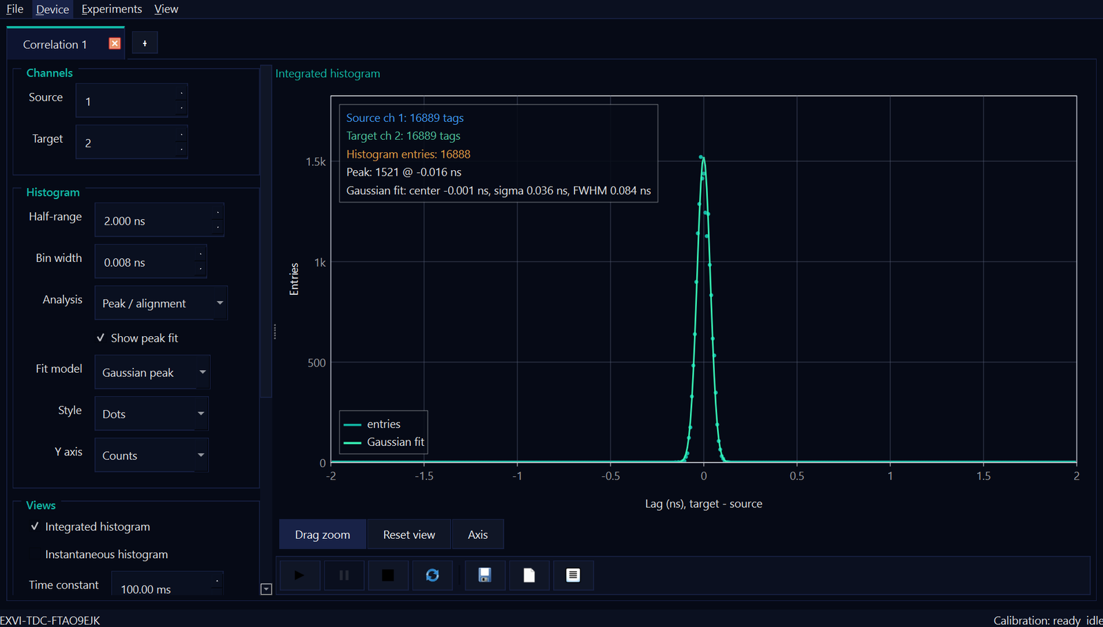
The GUI + SDK package for the TDC-A time tagger. Configure channels and thresholds, watch live counts and correlation histograms, then script the same measurements from Python or C++. One installer covers all of it.
Software and tools to control Exvi's timing devices.
Set up channels and thresholds, watch live counts and correlation histograms, and save data — no code required.
Drive the instrument and pull timestamps from automated experiments, measurement systems, and custom analysis. The API ships inside every installer, alongside the GUI.
USB support for the FTDI module used by the instrument. Windows uses the official FTDI VCP installer; on Linux, FTDI VCP support is built into the kernel.
exvi.timing v0.3.0 — installers for Windows, Linux, and Android (desktop GUI plus the Python & C++ API).
Live timing view with counts, streaming, and correlation histograms — plug in over USB and start measuring.
exvi.timing — the Correlation experiment: a live cross-correlation histogram with Gaussian peak fit, timing statistics, and per-experiment controls.
The Python and C++ APIs share one object model and the same method names. Full reference in the user manual, §7.
import exvi.timing as tt

# Connect to the first available TDC-A
dev = tt.Device.open_first()

# Set input thresholds (volts)
dev.set_thresholds([0.5, 0.5, 0.5, 0.5])

# On-device counts over a 1 s gate
r = dev.count_for(1.0)
print(f"IN1 rate: {r.rate_hz(tt.Input.IN1):.0f} counts/s")

dev.close()
#include "exvi/timing.hpp"
#include <iostream>
using namespace std::chrono_literals;
namespace tt = exvi::timing;

int main() {
    tt::Device dev = tt::Device::open_first();

    // Set input thresholds (volts)
    dev.set_thresholds({0.5, 0.5, 0.5, 0.5});

    // On-device counts over a 1 s gate
    auto r = dev.count_for(1s);
    std::cout << "IN1 rate: "
              << r.rate_hz(tt::Input::IN1)
              << " counts/s\n";
    return 0;
}
Current software support is provided for Windows and Linux. macOS support may be added later.
A time tagger records the precise arrival time of electrical pulses — one timestamp per event, at picosecond resolution. Instead of averaging a signal, you keep every event, which is what makes correlation, lifetime, and coincidence-style analysis possible in software.
A time tagger — also called a time-to-digital converter (TDC) — timestamps the moment a signal crosses a threshold on each of its inputs. Every event becomes a (channel, time) pair with picosecond resolution. Because nothing is thrown away or averaged in hardware, you can reconstruct timing statistics afterwards: rates, delay histograms, correlations, lifetimes, and coincidence-style relationships between channels.
It sits between your detectors (single-photon detectors, PMTs, SiPMs, discriminators, logic outputs) and your computer: the detectors produce electrical pulses, the tagger turns those pulses into calibrated timestamps, and your software does the physics.
Each event is stamped with an absolute time in picoseconds. The bin size is the finest time step the device can distinguish; on the TDC-A it is configurable down to 4 ps.
The run-to-run spread of a timestamp. It sets how sharply two events can be resolved in time — the TDC-A is ~22 ps RMS (typical). It is the quantity a cross-correlation width actually measures.
A short blind interval after each accepted event. It caps the maximum event rate and can be used deliberately to suppress detector after-pulses or re-triggering.
Two streamed events “coincide” when they fall within a chosen time window. This host-side analysis is the foundation of correlation, heralding, and entanglement measurements.
A histogram of the delays between two channels reveals their timing relationship: the peak position is the relative delay, its width is the combined jitter. In quantum optics this is the second-order correlation g²(τ).
Locking the timebase to an external 10 MHz or 1 PPS reference bounds long-term drift and gives a common, traceable time across several instruments.
Have a review paper we should list here? Email info@exvi.io.
Concrete measurements the TDC-A is built for. Each follows the same pattern: threshold the inputs, stream calibrated time tags, and compute the result on the host with the Python or C++ API. Correlations and histograms are done host-side from the tag stream.
What it is. A Hanbury Brown–Twiss (HBT) measurement: send a source onto two detectors and histogram the delays between their clicks. The second-order correlation g²(τ) characterizes the source — a dip to g²(0) < 0.5 signals single-photon emission (antibunching); for photon-pair sources, the correlation peak quantifies the pairs and heralding efficiency.
With the TDC-A. Connect the two detectors to two inputs, stream time tags, and build the cross-correlation histogram of the click delays.
import exvi.timing as tt
import numpy as np

dev = tt.Device.open_first()
dev.set_thresholds([0.5, 0.5, 0.0, 0.0])          # detectors on IN1, IN2
dev.start_tag_stream([tt.Input.IN1, tt.Input.IN2])

t1, t2 = [], []
for _ in range(2000):                             # collect a batch of tags
    for tag in dev.read_tags(8192, timeout_seconds=0.1):
        (t1 if tag.input == tt.Input.IN1 else t2).append(tag.timestamp_ps)

dev.stop_tag_stream(); dev.close()

# cross-correlate the two click trains -> g2(tau) around zero delay
# (build a histogram of t2 - t1 for nearby pairs; dip at 0 = antibunching)
What it is. Measure how long a fluorophore stays excited by histogramming photon arrival times relative to the laser pulse that excited it. The decay histogram, fit to an exponential, gives the fluorescence lifetime τ; scanning the sample turns those lifetimes into an image (FLIM).
With the TDC-A. Feed the laser sync into one input and the detector into another; histogram detector arrivals relative to the preceding sync pulse (a start–stop measurement). For imaging, index the histograms by the scanner's pixel marker.
import exvi.timing as tt

dev = tt.Device.open_first()
dev.set_thresholds([1.0, 0.5, 0.0, 0.0])          # IN1 = laser sync, IN2 = detector
dev.start_tag_stream([tt.Input.IN1, tt.Input.IN2])

# for each detector tag, record its delay after the most recent sync tag;
# accumulate those delays into a histogram -> the fluorescence decay curve,
# then fit an exponential for the lifetime tau.

dev.stop_tag_stream(); dev.close()
What it is. Characterize an oscillator, GPS-disciplined reference, or 1 PPS by timestamping its edges against the tagger's timebase — measure period, jitter, drift, or Allan deviation, optionally with the TDC-A locked to a traceable 10 MHz reference.
With the TDC-A. Feed the clock or 1 PPS into an input, timestamp its edges, and compute the statistics from the inter-edge intervals.
import exvi.timing as tt
import numpy as np

dev = tt.Device.open_first()
dev.set_clock(tt.ClockSource.CLKIN)               # lock to a 10 MHz reference (optional)
dev.set_thresholds([1.5, 0.0, 0.0, 0.0])          # clock / 1 PPS on IN1
dev.start_tag_stream([tt.Input.IN1])

edges = []
for _ in range(2000):
    edges += [t.timestamp_ps for t in dev.read_tags(8192, timeout_seconds=0.1)]

dev.stop_tag_stream(); dev.close()

periods = np.diff(edges)
print(f"period {np.mean(periods)/1e3:.3f} ns, jitter {np.std(periods):.1f} ps")
We're expanding these into step-by-step guides with wiring diagrams and complete analysis code. Tell us which one you need first.
Fun things to do with a TDC-A. Some run today; some we're still building. Ideas welcome — tell us what you'd like to see.
Stream calibrated time tags over USB to an Android phone, then forward them over local Wi-Fi to a workstation or cluster for processing. Any bench becomes a distributed acquisition node — the instrument stays tiny while the compute lives wherever you want it. (Android support is on the roadmap.)
A few lines of Python that print real-time count rates on each input — the “hello world” of a time tagger, and a quick way to confirm your setup is wired correctly.
A quick g²(0) check with two detectors (HBT). Watch the dip at zero delay drop below 0.5 as your source gets cleaner — the classic antibunching signature, live.
Feed a 1 PPS or clock edge into an input and watch its period and jitter update live — a cheap way to eyeball an oscillator or a GPS-disciplined reference.
Two scintillator + SiPM paddles in coincidence: when both fire within a few nanoseconds, you (probably) caught a muon passing through. A classroom-friendly particle detector on a USB budget.
We'd love to hear it — and we're happy to feature community projects. Get in touch.
Base prices are listed per device on the product pages — you shouldn't have to request a quote just to find out what an instrument costs.
The TDC-A is not yet available for general sale. It is completing conformity assessment (CE / UKCA / FCC). Ahead of certification, a limited number of evaluation prototypes are available to early partners for testing and integration — supplied as pre-production units for evaluation only. To enquire about a prototype, use the General questions form or email info@exvi.io.
Compatibility, applications, lead time, software, or anything else.
These Terms & Conditions ("Terms") govern use of this website and the sale of products and software by Exvi Technologies, LLC ("Exvi", "we", "us"), California, USA. By using the site, requesting a quotation, or placing an order, you agree to these Terms. Where a signed agreement or a firm quotation states different terms, that document controls for that transaction.
Last updated: 19 June 2026. We may update these Terms from time to time; the version in effect at the time of your order applies.